Quick start
This walkthrough mirrors the 13-step quick start in the official manual. It uses the bundled
sample file STO.xlsx (SrTiO₃ thin film, Thermo Kalpha) found in the Data/ folder.
1. Instrument settings
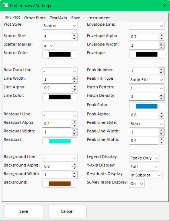
Before analysis, set the correct sensitivity factor library. Open Edit → Preferences → Instrument Settings and pick the entry for your instrument:
- General:
C-Al1486andTPP-2M - Thermo Kalpha / Nexsa:
A-ALTHERMO1andTPP-2M - Kratos (newer):
C-KRATOSF1S - Al1486andTPP-2M - Kratos (older):
C-KRATOSC1S - Al1486andTPP-2M
The X-ray-to-analyser angle defaults to the magic angle (54.7°). Doublet splittings live in C-Al1486 and apply across all instruments.
2. Open files
Drag any supported XPS file (.xlsx, .vms, .kal, .spe, …) into the plot area. If the
file is not already in KherveFitting format, the program creates an Excel file in the
correct format with corrected raw data and exported transmission. Multiple files can be
dragged at once.
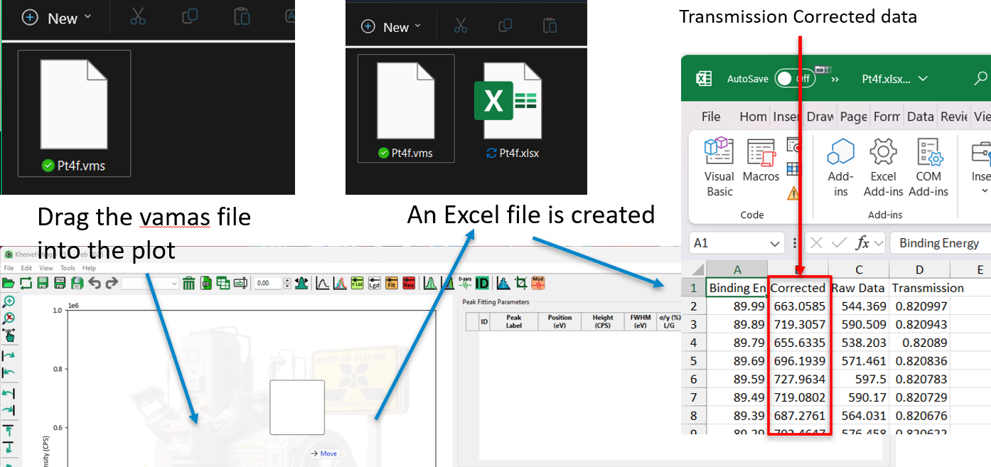
For this walkthrough, drag STO.xlsx from the Data folder and use the middle mouse
wheel to scroll to the Sr3d core level. Make sure RSF library A-ALTHERMO1 is selected.
3. Plot and core-level control
A few essential shortcuts:
- Mouse wheel — switch between core levels (or
Ctrl+[/Ctrl+]) - Ctrl+←/→ — pan along the X axis
- Ctrl+↑/↓ — zoom Y
- Ctrl + + / Ctrl + − — zoom X
- Ctrl+Shift+← — zoom X while keeping the low-BE minimum constant
4. Prepare for peak fitting
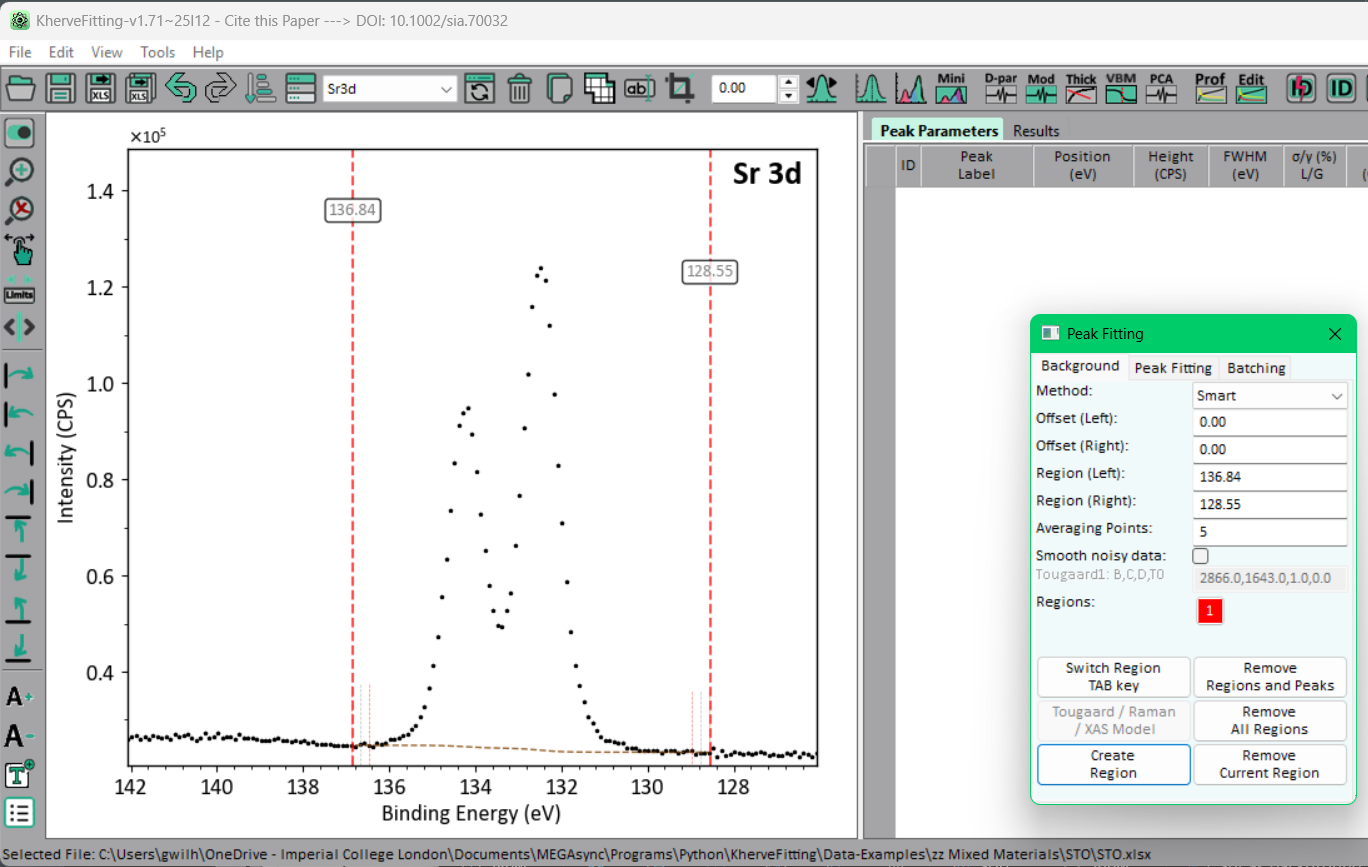
Click the peak-fit icon to open the fitting window. It has two tabs: Background and Peak Fitting. Default fitting method is least squares; default model is GL (Area) — adequate for newcomers, but Voigt (Area, L/G, σ) is recommended for physical meaningfulness. LA (Area, σ/γ, γ) is familiar to CasaXPS users.
5. Create a background
Click on the left (high BE) and right (low BE) of the plot, ideally in flat regions 1–2 eV away from peaks, then press Create Region. With Smart or Shirley, a Shirley background is generated and labelled region "1".
6. Create a peak model
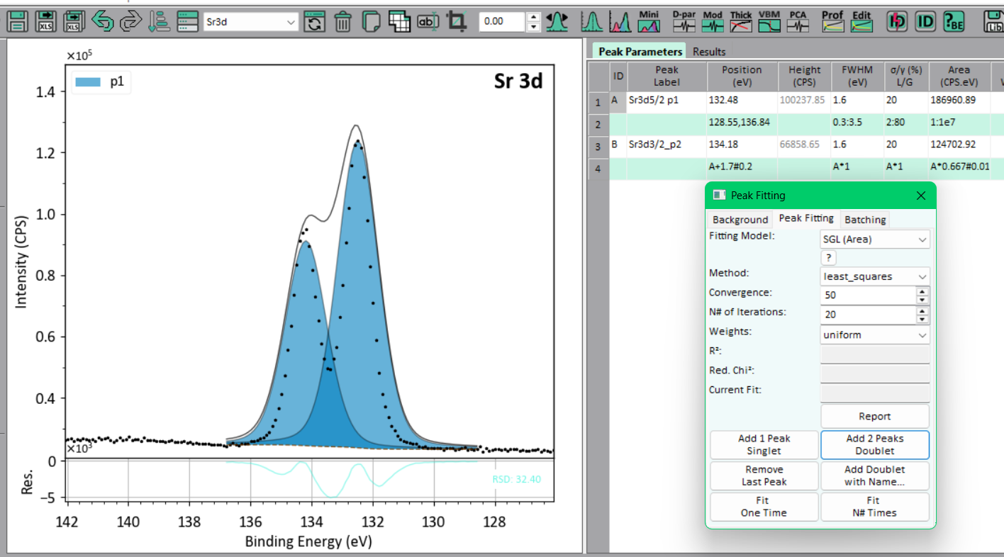
Switch to the Peak Fitting tab. The Sr3d core level is a doublet (~1 eV FWHM, split by ~1.7 eV). Press Add 2 Peaks. Two peaks A and B are created with peak B linked to A:
- Position
A + 1.7 # 0.2— B is 1.7 eV from A, ±0.2 eV variation - FWHM
A × 1— locked equal to A - Area
A × 0.667 # 0.05— d-shell ratio (4/6) ±0.05
7. Fit the peak model
Press Fit N# times and wait for the iterations. RSD around 2.0–3.4 is acceptable for an SGL fit. You'll see FWHM ~1.0 eV and L/G ~62 %.
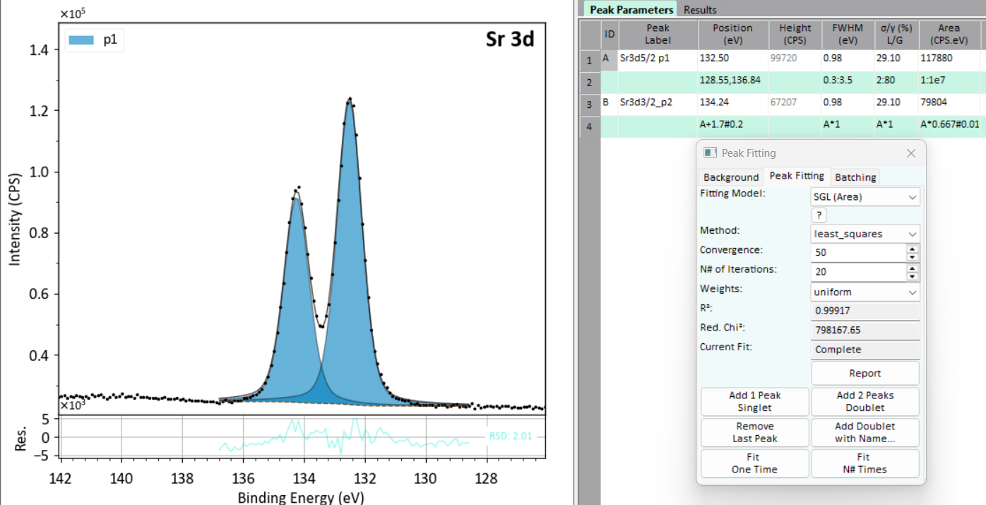
Sharper peaks tend more Lorentzian; broader peaks tend more Gaussian. Avoid fixing shape at 30 % across all peaks.
8. Move the peak model
Press Tab or Q to select peak A. With the cursor on the cross marker, drag A — peak B follows because it's linked. To move B alone, drag B directly. Alt + arrow keys also nudge a selected peak.
9. Other models — LA and Voigt
Remove the SGL pair, switch to LA, fit again — RSD ~1.8–2.4. The LA model is a full Lorentzian powered on the right by γ and on the left by σ; σ/γ controls asymmetry (50 % = symmetric).
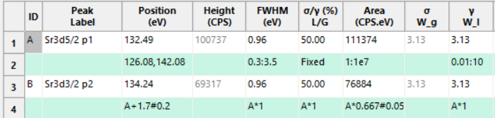
Switch to Voigt and refit — RSD ~2.9–3.1. Unlike GL/LA, the Voigt FWHM cannot be constrained directly: you constrain Gaussian width and L/G ratio, and the Lorentzian width follows. Rules of thumb:
- FWHM 1.0–1.5 eV ⇒ L/G ~20 %
- FWHM > 1.5 eV ⇒ L/G ~10–20 %
- FWHM < 1.0 eV ⇒ L/G rises sharply to 50–60 %
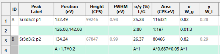
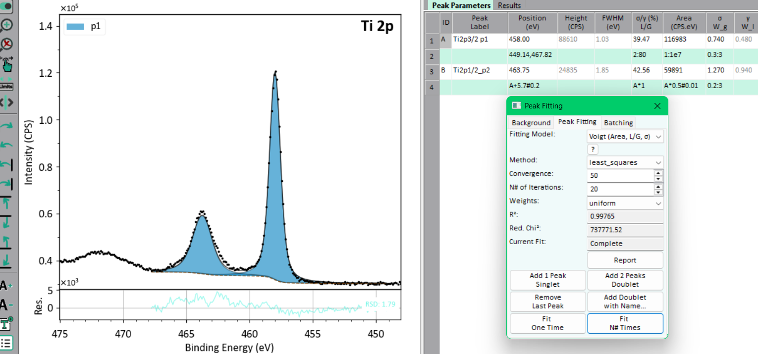
Repeat the fit on Ti2p with the Voigt model. KherveFitting does not lock B's FWHM to A for Ti2p / V2p — Ti2p₁/₂ is broader than Ti2p₃/₂ for oxides due to the Köster-Kronig effect.
10. Export to Results Grid
With the correct RSF library set, press the Export icon to push the fit to the Results grid. Tick Ti2p₃/₂ and Sr3d₅/₂ to compare atomic concentrations.

11. Load a peak table
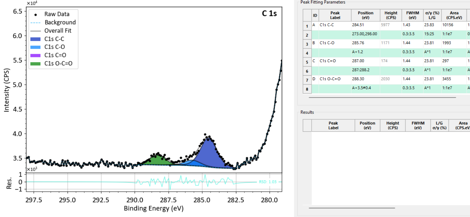
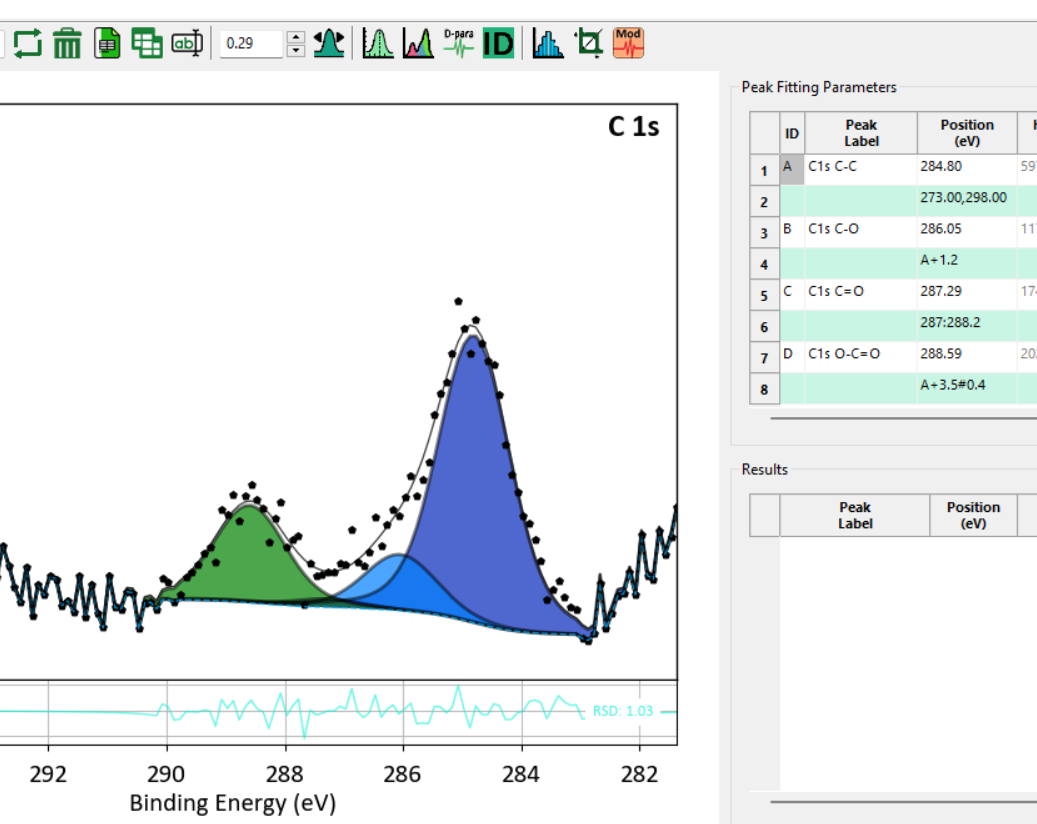
Saved peak tables are JSON. Scroll to C 1s, press Load Peaks Parameter in the
horizontal toolbar, and pick C1s_C-C_4peaks_Voigt_GK_xxxx.json. Four peaks appear in the
fitting grid. Place a Shirley background, fit — RSD around 1 should result.
Repeat on O 1s with O1s_O-Lat_3peaks_Voigt_GK_xxxx.json (background between 527.3 and
535 eV; the O-surf peak is often negligible and can be removed).
12. Binding energy correction
KherveFitting looks for a peak named C1s C-C and computes the offset to 284.8 eV (this
target is configurable in Preferences → Instrument Settings). Click the green BE-correction
button — every peak in the fitting and Results grids shifts by the same amount. Type 0.00
and click the plot to revert.
13. Background offset
Scroll to O 1s, zoom down with Ctrl+↓ to background level. On the Background tab, reset vertical lines, choose 527.3–537.5 eV, hold Shift, and drag the high-BE side of the background down to fine-tune.
What's next
- Background models — when to use Shirley vs Tougaard vs Linear
- Peak models — full list of fitting line shapes
- Depth profiling — running a sputter series end-to-end